Multiple runs

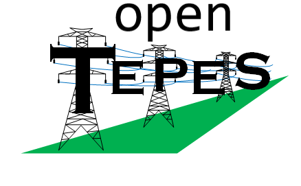
Many studies run the same model over many related cases — scenario ensembles, demand or fuel-cost scans, Monte-Carlo samples. openTEPES offers three modes for this, trading set-up cost for reuse, all driven by one orchestrator (openTEPES_Runner.run). A single-case run reproduces a direct openTEPES_run.

The code calls a set of related runs a sweep: openTEPES_Runner is the sweep runner, the three modes below are the sweep modes A/B/C, and the merged output tables are named oT_Sweep_*.

Mode	What each worker repeats	Cost per case	When to use
A — pre-build	read input + build + solve	full	cases that differ structurally, each in its own folder
B — in-memory overlay	build + solve (input read once)	build + solve	one baseline perturbed by a scale factor or a table patch
C — post-build hot-swap	solve only (built once)	solve	one built model re-solved over a range of parameter values

Mode A — pre-build sweep

Each case reads its own input source, builds its own model, solves, and writes its own results. It is the most general mode: the cases may differ in any way, since nothing is shared between them.

A Case names one input source (a CSV case directory or a .duckdb file) plus an optional output directory and label. Cases that share the same (dir_name, case_name) need distinct out_path values so their result writers do not collide.

from openTEPES import openTEPES_Cases, openTEPES_Runner

cases = [
    openTEPES_Cases.Case("cases", "SE2035_low"),
    openTEPES_Cases.Case("cases", "SE2035_ref"),
    openTEPES_Cases.Case("cases", "SE2035_high"),
]

summary = openTEPES_Runner.run(cases, solver_name="gurobi",
                               mode="pre-build", backend="multiprocessing", n_workers=8)

Backends. backend="serial" (default, no extra dependency) runs the cases one after another; "multiprocessing" spreads them across a standard-library Pool of n_workers; "joblib" uses joblib.Parallel (an optional dependency — pip install joblib). All three preserve input order in the returned list.

Results come back as summaries, not models. A Pyomo model cannot cross a worker-process boundary, so each worker writes its results to disk and run reads back that case’s openTEPES_run_status_*.json, returning one summary dict per case. A case that raises is captured as status="error", so one failure does not abort the run.

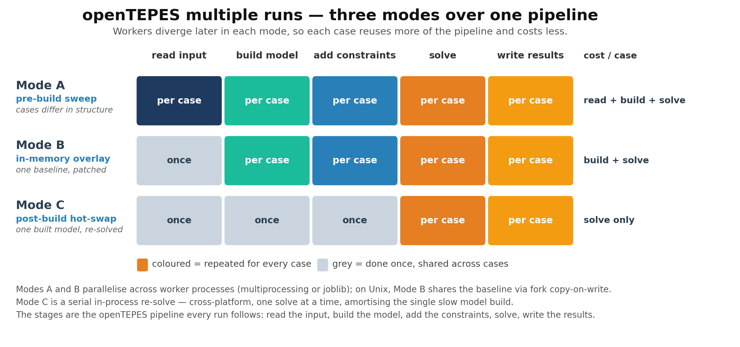
Mode B — in-memory overlay

When every case starts from one baseline, re-reading the input for each is wasteful. Mode B reads the baseline once into memory and re-uses it, so the run pays the input I/O once and only rebuilds and solves per case.

How the baseline is shared. The runner calls InMemorySource.materialize(open_source(path)) once per distinct baseline, holding every input table in RAM as a DataFrame. Each case gets a cheap clone via with_overlay(...) that shares those frames. Under the multiprocessing backend on Unix the workers are forked, so they see the baseline through copy-on-write — no extra memory, no re-read. On Windows the baseline is pickled once per task instead (still no CSV re-read, just without the copy-on-write saving). Mode B needs a distinct out_path per case, since the cases share the baseline directory.

The overlay maps a data-table stem (e.g. "Demand") to one of:

• a number — multiply every numeric value of that table (a uniform scale, 1.10 for +10 %);

• a df -> df callable — any transform of the baseline frame;

• a replacement DataFrame — swap the table outright (in the wide, indexed shape the model reads).

Overlays target the oT_Data_* tables; the dimension tables pass through unchanged. An empty overlay reproduces a direct run exactly.

openTEPES_Runner.run(
    [openTEPES_Cases.Case("cases", "SE2035_base", out_path="out/d105", overlay={"Demand": 1.05}),
     openTEPES_Cases.Case("cases", "SE2035_base", out_path="out/d110", overlay={"Demand": 1.10})],
    solver_name="gurobi", mode="in-memory", backend="multiprocessing", n_workers=8)

The diagram below traces one such run.

Mode C — post-build hot-swap

Mode C is the cheapest and, despite handling the largest runs, the simplest in code: it builds the model once and only re-solves it, one overlay at a time. It is a plain serial loop in a single process — no worker pool, no forking — so it runs unchanged on every platform. Its speed comes not from parallelism but from skipping the rebuild, the slowest step on large cases. It is driven directly by openTEPES_ProblemSolvingResolve.resolve, not through openTEPES_Runner.

from openTEPES.openTEPES_ProblemSolvingResolve import resolve, overlay_scaled

# OptModel is an already-built model (from openTEPES_run's build step)
results = resolve(OptModel, "gurobi",
                  overlays=[overlay_scaled(OptModel, "pDemandElec", 1.05),
                            overlay_scaled(OptModel, "pDemandElec", 1.10)])

How the hot-swap works. Each overlay is a dict mapping a Param name to new values. For each overlay, resolve writes the new numbers into the built model with Param.store_values(...) and re-solves. This works only for Params declared mutable=True, so Mode C sweeps the operational set only — pDemandElec, pENSCost, pLinearVarCost, pEFOR, pReserveMargin, pRESEnergy. Structural and topology Params stay immutable (a mutable Param read in a build-time if would raise), so anything that changes the model’s structure needs Mode A or B.

The solver must be non-persistent. resolve makes a fresh SolverFactory(SolverName); a non-persistent solver re-exports the model from the current Param values on every solve, so store_values takes effect with no extra call. Pass a plain solver name ("gurobi", "highs"), not a persistent one.

Overlays are independent, not cumulative. resolve snapshots the baseline of every touched Param and resets to it before each overlay, so overlay k does not build on overlay k−1. An empty overlay {} re-solves the baseline; restore=True (default) restores the baseline at the end. overlay_scaled(model, name, factor) builds a scale-factor overlay for one Param.

resolve returns one dict per overlay with the solver termination condition and the total system cost (None if the solve was not optimal). It solves one overlay at a time; to run a large Monte-Carlo in parallel, wrap resolve in your own worker pool.

Collecting sweep results

openTEPES_ResultAggregate.aggregate stacks a sweep’s cases into one long table per result, with a leading case column, reading either the per-case DuckDB files or the per-case CSV folders:

from openTEPES.openTEPES_ResultAggregate import aggregate

aggregate(sources=["out/d105", "out/d110"], out_path="out/sweep", to="duckdb")

openTEPES_Runner.run can do this in one step with aggregate_to=.... Per-case DuckDB output keeps a sweep single-writer-safe (one database per case). See Output Results for the output_format option that writes those per-case DuckDB files.